Echoregions Regions2D Plotting Demonstration

Prior to running this notebook and all other notebooks, make sure you have installed the packages found in requirements.txt.

This notebook demonstrates some of the functionalities of echoregions to read Echoview region .evr files and visualize regions.

import matplotlib.pyplot as plt
import xarray as xr
from datetime import timedelta
import echoregions as er
import warnings
import gdown
import urllib.request

warnings.filterwarnings("ignore", category=DeprecationWarning)

# download an example file
urllib.request.urlretrieve("https://raw.githubusercontent.com/OSOceanAcoustics/echoregions/main/echoregions/test_data/x1.evr","x1.evr")

EVR_FILE = 'x1.evr'

Get a Regions2D object with read_evr

r2d = er.read_evr(EVR_FILE)

Plotting

# Display availible regions
print(r2d.data.region_id.values)

<IntegerArray>
[ 1,  2,  3,  4,  5,  6,  7,  8,  9, 10, 11, 12, 13, 14, 15, 16, 17, 18, 19,
 20, 22, 23, 24, 25, 26, 27, 28, 29, 30, 32, 33, 34, 35]
Length: 33, dtype: Int64

# let's select one id
region_id = 11

# Plot a region with a specific id with the `plot` function
r2d.plot(region_id)

# Plot a closed region by using close_region=True.
# Optionally provide matplotlib kwargs for more customization.
r2d.plot(region_id, close_region=True, color='k', alpha=.5, marker='x', markeredgecolor='red', markersize=12)

Plotting regions on an echogram

Reading Preprocessed Sonar Files

We have converted and calibrated a sample of echosounder files from the same transect and stored them in .nc. We can directly read them with the xarray library.

# mounting the google drive (uncomment if you have permission to read directly from Google Drive)
# from google.colab import drive
# drive.mount('/content/drive/') 

# Paths for Google Drive read  (uncomment if you have permission to read directly from Google Drive)
# SONAR_PATH_Sv = '/content/drive/Shareddrives/uw-echospace/shared_data/SH1707/sample/Sv/'
# SONAR_PATH_raw = '/content/drive/Shareddrives/uw-echospace/shared_data/SH1707/sample/raw_converted/'

# download a zipped sample folder from publicly available Google Drive
url = 'https://drive.google.com/uc?id=1OhYVcakCEgXEKA4R9za4jvBWQUFIOnE5'
output = 'x1.tar.gz'
gdown.download(url, output, quiet=False)

# unzip into a sample folder
!tar -xvzf  x1.tar.gz

ds = xr.open_dataset("x1.zarr")

c:\Users\cmtug\OneDrive\Documents\GitHub\echoregions\.conda\lib\site-packages\xarray\backends\plugins.py:139: RuntimeWarning: 'netcdf4' fails while guessing
  warnings.warn(f"{engine!r} fails while guessing", RuntimeWarning)
c:\Users\cmtug\OneDrive\Documents\GitHub\echoregions\.conda\lib\site-packages\xarray\backends\plugins.py:139: RuntimeWarning: 'h5netcdf' fails while guessing
  warnings.warn(f"{engine!r} fails while guessing", RuntimeWarning)
c:\Users\cmtug\OneDrive\Documents\GitHub\echoregions\.conda\lib\site-packages\xarray\backends\plugins.py:139: RuntimeWarning: 'scipy' fails while guessing
  warnings.warn(f"{engine!r} fails while guessing", RuntimeWarning)

The dataset has a range_sample dimension and instead we convert it to a depth dimension by adjusting the water level.

# create depth coordinate:
echo_range = ds.echo_range.isel(channel=0, ping_time=0)
# assuming water levels are same for different frequencies and location_time
depth = ds.water_level.isel(channel=0, ping_time=0) + echo_range
depth = depth.drop_vars('channel')
# creating a new depth dimension
ds['depth'] = depth
ds = ds.swap_dims({'range_sample': 'depth'})

ds.Sv

<xarray.DataArray 'Sv' (channel: 3, ping_time: 13192, depth: 3957)>
[156602232 values with dtype=float64]
Coordinates:
  * channel       (channel) object 'GPT  18 kHz 009072058c8d 1-1 ES18-11' ......
  * depth         (depth) float64 9.15 9.15 9.15 9.34 ... 758.1 758.3 758.5
  * ping_time     (ping_time) datetime64[ns] 2017-06-25T15:04:30.076000256 .....
    range_sample  (depth) int64 0 1 2 3 4 5 6 ... 3951 3952 3953 3954 3955 3956

xarray.DataArray

'Sv'

• channel: 3
• ping_time: 13192
• depth: 3957

• ...

  [156602232 values with dtype=float64]

• Coordinates: (4)
  • channel
    (channel)
    object
    'GPT 18 kHz 009072058c8d 1-1 ES...

    array(['GPT  18 kHz 009072058c8d 1-1 ES18-11',
           'GPT  38 kHz 009072058146 2-1 ES38B',
           'GPT 120 kHz 00907205a6d0 4-1 ES120-7C'], dtype=object)

  • depth
    (depth)
    float64
    9.15 9.15 9.15 ... 758.3 758.5

    array([  9.15    ,   9.15    ,   9.15    , ..., 758.133532, 758.323052,
           758.512572])

  • ping_time
    (ping_time)
    datetime64[ns]
    2017-06-25T15:04:30.076000256 .....

    array(['2017-06-25T15:04:30.076000256', '2017-06-25T15:04:33.959000064',
           '2017-06-25T15:04:37.832999936', ..., '2017-06-26T02:20:02.698999808',
           '2017-06-26T02:20:05.571999744', '2017-06-26T02:20:08.442999808'],
          dtype='datetime64[ns]')

  • range_sample
    (depth)
    int64
    0 1 2 3 4 ... 3953 3954 3955 3956

    array([   0,    1,    2, ..., 3954, 3955, 3956], dtype=int64)

• Indexes: (3)
  • channel
    PandasIndex

    PandasIndex(Index(['GPT  18 kHz 009072058c8d 1-1 ES18-11',
           'GPT  38 kHz 009072058146 2-1 ES38B',
           'GPT 120 kHz 00907205a6d0 4-1 ES120-7C'],
          dtype='object', name='channel'))

  • depth
    PandasIndex

    PandasIndex(Index([ 9.149999618530273,  9.149999618530273,  9.149999618530273,
            9.339519743051781,  9.529039867573289,  9.718559992094796,
            9.908080116616304, 10.097600241137812,  10.28712036565932,
           10.476640490180827,
           ...
            756.8068908558781,  756.9964109803996,  757.1859311049211,
            757.3754512294427,  757.5649713539641,  757.7544914784856,
            757.9440116030071,  758.1335317275286,  758.3230518520502,
            758.5125719765716],
          dtype='float64', name='depth', length=3957))

  • ping_time
    PandasIndex

    PandasIndex(DatetimeIndex(['2017-06-25 15:04:30.076000256',
                   '2017-06-25 15:04:33.959000064',
                   '2017-06-25 15:04:37.832999936',
                   '2017-06-25 15:04:41.708000256',
                   '2017-06-25 15:04:45.593999872',
                   '2017-06-25 15:04:49.468000256',
                      '2017-06-25 15:04:53.344000',
                   '2017-06-25 15:04:57.229000192',
                      '2017-06-25 15:05:01.104000',
                   '2017-06-25 15:05:04.977999872',
                   ...
                   '2017-06-26 02:19:42.717000192',
                   '2017-06-26 02:19:45.590000128',
                   '2017-06-26 02:19:48.410999808',
                   '2017-06-26 02:19:51.295000064',
                   '2017-06-26 02:19:54.168999936',
                   '2017-06-26 02:19:56.993999872',
                   '2017-06-26 02:19:59.817999872',
                   '2017-06-26 02:20:02.698999808',
                   '2017-06-26 02:20:05.571999744',
                   '2017-06-26 02:20:08.442999808'],
                  dtype='datetime64[ns]', name='ping_time', length=13192, freq=None))

• Attributes: (0)

Plotting

# plot Sv
ds.Sv.isel(channel=0).plot(x='ping_time', vmax=-40, vmin=-100, yincrease=False, figsize=(20,8))
# plot region
r2d.plot(region_id, close_region=True, color='k')
plt.show()

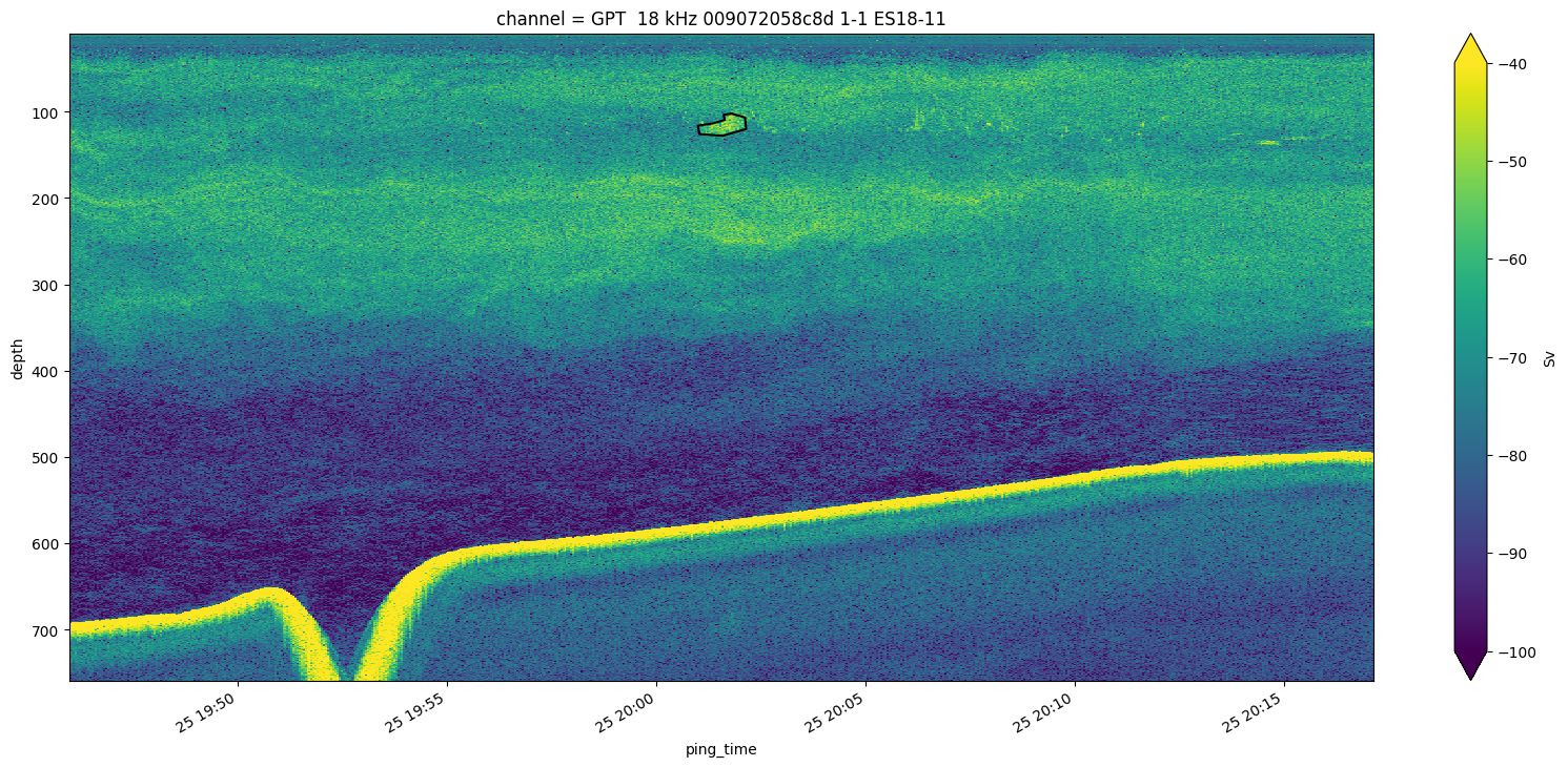
Let’s limit the time extent of the echogram so that we can see better the region.

# we will create a 15 minute window around the bounding box of the region
bbox_right = r2d.data[r2d.data.region_id==region_id].region_bbox_right.iloc[0] + timedelta(minutes = 15)
bbox_left = r2d.data[r2d.data.region_id==region_id].region_bbox_left.iloc[0] - timedelta(minutes = 15)

# plot Sv
ds.Sv.isel(channel=0).sel(ping_time=slice(bbox_left, bbox_right)).plot(x='ping_time', vmax=-40, vmin=-100, yincrease=False, figsize=(20,8))
# plot region
r2d.plot(region_id, close_region=True, color='k')
plt.show()