Echoregions Regions2D Plotting and Masking Demonstration

Echoregions Regions2D Plotting and Masking Demonstration#

Prior to running this notebook and all other notebooks, make sure you have installed the packages found in requirements.txt.

This notebook demonstrates some of the functionalities of echoregions to read Echoview region .evr files and visualize regions.

import matplotlib.pyplot as plt
import xarray as xr
import numpy as np
import echoregions as er
import warnings
import urllib.request
import gdown

warnings.filterwarnings("ignore", category=DeprecationWarning)

# download an example file
urllib.request.urlretrieve("https://raw.githubusercontent.com/OSOceanAcoustics/echoregions/main/echoregions/test_data/x1.evr","x1.evr")

EVR_FILE = 'x1.evr'

Get a Regions2D object with `read_evr`#

r2d = er.read_evr(EVR_FILE)

Plotting#

# Display availible regions
r2d.data.region_id.values

<IntegerArray>
[ 1,  2,  3,  4,  5,  6,  7,  8,  9, 10, 11, 12, 13, 14, 15, 16, 17, 18, 19,
 20, 22, 23, 24, 25, 26, 27, 28, 29, 30, 32, 33, 34, 35]
Length: 33, dtype: Int64

# let's select one id
region_ids = [11]

# Plot a region with a specific id with the `plot` function
r2d.plot(region_ids[0])

_images/f4ca8a3e5f5bab4f4ac113aeeb49d886edd450b26c50b0827e80b9b42d2ea2fe.png

# Plot a closed region by using close_region=True.
# Optionally provide matplotlib kwargs for more customization.
r2d.plot(region_ids[0], close_region=True, color='k', alpha=.5, marker='x', markeredgecolor='red', markersize=12)

_images/ccddf506d86fcd635c797a1202882de7225347e06a97b60d279fec6ee12a4c19.png

r2d.select_region(region_ids)

	file_name	file_type	evr_file_format_number	echoview_version	region_id	region_structure_version	region_point_count	region_selected	region_creation_type	dummy	...	region_bbox_right	region_bbox_top	region_bbox_bottom	region_class	region_type	region_name	time	depth	region_notes	region_detection_settings
10	x1	EVRG	7	12.0.341.42620	11	13	10	0	2	-1	...	2017-06-25 20:02:08.535700	102.255201	127.947603	Unknown	1	Chicken nugget	[2017-06-25T20:01:47.093000000, 2017-06-25T20:...	[102.2552007996, 103.7403107496, 109.532239554...	[]	[]

1 rows × 22 columns

Plotting regions on an echogram#

Reading Preprocessed Sonar Files#

We have converted and calibrated the echosounder files corresponding to one transect and stored them in .zarr. We can directly read them with the xarray library.

# mounting the google drive (uncomment if you have permission to read directly from Google Drive)
# from google.colab import drive
# drive.mount('/content/drive/') 

# Paths for Google Drive read  (uncomment if you have permission to read directly from Google Drive)
# ZARR_PATH = '/content/drive/Shareddrives/uw-echospace/shared_data/SH1707/x1.zarr'

# download a zipped sample folder from publicly available Google Drive
url = 'https://drive.google.com/uc?id=1OhYVcakCEgXEKA4R9za4jvBWQUFIOnE5'
output = 'x1.tar.gz'
gdown.download(url, output, quiet=False)

# Unzip into a sample folder
!tar -xvzf  x1.tar.gz

tar: Error opening archive: Failed to open 'x1.tar.gz'

ds = xr.open_dataset("x1.zarr")

c:\Users\cmtug\OneDrive\Documents\GitHub\echoregions\.conda\lib\site-packages\xarray\backends\plugins.py:139: RuntimeWarning: 'netcdf4' fails while guessing
  warnings.warn(f"{engine!r} fails while guessing", RuntimeWarning)
c:\Users\cmtug\OneDrive\Documents\GitHub\echoregions\.conda\lib\site-packages\xarray\backends\plugins.py:139: RuntimeWarning: 'h5netcdf' fails while guessing
  warnings.warn(f"{engine!r} fails while guessing", RuntimeWarning)
c:\Users\cmtug\OneDrive\Documents\GitHub\echoregions\.conda\lib\site-packages\xarray\backends\plugins.py:139: RuntimeWarning: 'scipy' fails while guessing
  warnings.warn(f"{engine!r} fails while guessing", RuntimeWarning)

The dataset has a range_sample dimension and instead we convert it to a depth dimension by adjusting the water level.

# create depth coordinate:
echo_range = ds.echo_range.isel(channel=0, ping_time=0)
# assuming water levels are same for different frequencies and location_time
depth = ds.water_level.isel(channel=0, ping_time=0) + echo_range
depth = depth.drop_vars('channel')
# creating a new depth dimension
ds['depth'] = depth
ds = ds.swap_dims({'range_sample': 'depth'})

# set the min and max depth based on the sonar files
r2d.min_depth = ds.depth.min()
r2d.max_depth = ds.depth.max()

r2d.select_region(region_ids[0])

	file_name	file_type	evr_file_format_number	echoview_version	region_id	region_structure_version	region_point_count	region_selected	region_creation_type	dummy	...	region_bbox_right	region_bbox_top	region_bbox_bottom	region_class	region_type	region_name	time	depth	region_notes	region_detection_settings
10	x1	EVRG	7	12.0.341.42620	11	13	10	0	2	-1	...	2017-06-25 20:02:08.535700	102.255201	127.947603	Unknown	1	Chicken nugget	[2017-06-25T20:01:47.093000000, 2017-06-25T20:...	[102.2552007996, 103.7403107496, 109.532239554...	[]	[]

1 rows × 22 columns

region_df = r2d.select_region(region_ids)

region_df

	file_name	file_type	evr_file_format_number	echoview_version	region_id	region_structure_version	region_point_count	region_selected	region_creation_type	dummy	...	region_bbox_right	region_bbox_top	region_bbox_bottom	region_class	region_type	region_name	time	depth	region_notes	region_detection_settings
10	x1	EVRG	7	12.0.341.42620	11	13	10	0	2	-1	...	2017-06-25 20:02:08.535700	102.255201	127.947603	Unknown	1	Chicken nugget	[2017-06-25T20:01:47.093000000, 2017-06-25T20:...	[102.2552007996, 103.7403107496, 109.532239554...	[]	[]

1 rows × 22 columns

region_ids

[11]

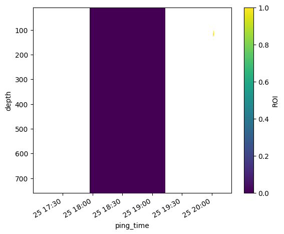
M = r2d.mask(ds.Sv.isel(channel=0).drop('channel'), region_ids, mask_var="ROI")

# the mask has nan's where outside of the region
M.shape

(3957, 13192)

# the region is labeled by default with 0 (if there are more regions they will be labeled 1,2,3,...)
M.max()

<xarray.DataArray 'ROI' ()>
array(0.)

# M.plot(yincrease=False)
# r2d.plot(region_ids, close_region=True, color='r')
M.sel(ping_time=slice('2017-06-25T20:00:00', '2017-06-25T20:20:00')).plot(yincrease=False)

<matplotlib.collections.QuadMesh at 0x2af21c755a0>

_images/800d44f154a1fa8b6d6a468e442beaabb13189893606ab093806b162c2c55a23.png

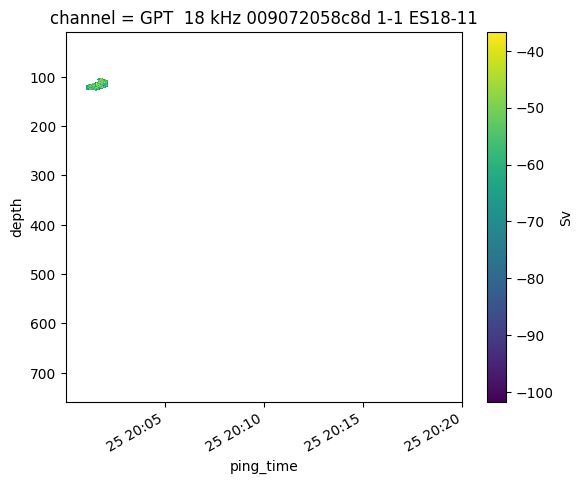
We can also create a masked sonar file:

Sv_masked = ds.Sv.where(~M.isnull())

# we limit the time range so that we see the small region
Sv_masked.sel(ping_time=slice('2017-06-25T20:00:00', '2017-06-25T20:20:00')).isel(channel=0).T.plot(yincrease=False)

<matplotlib.collections.QuadMesh at 0x2af21f2d960>

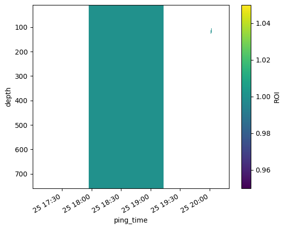
_images/c0a43d8572fc4e9ab0ca458c8366bbf9f8d74ada6cf07625176ca57d624c2e97.png

Multiple Region Mask#

The mask function can make a mask for several regions simultaneously:

region_ids = [10, 11]

r2d.select_region(region_ids)

	file_name	file_type	evr_file_format_number	echoview_version	region_id	region_structure_version	region_point_count	region_selected	region_creation_type	dummy	...	region_bbox_right	region_bbox_top	region_bbox_bottom	region_class	region_type	region_name	time	depth	region_notes	region_detection_settings
9	x1	EVRG	7	12.0.341.42620	10	13	4	0	4	-1	...	2017-06-25 19:13:12.607500	9.244758	758.973217	Side station	0	Region10	[2017-06-25T17:57:09.687500000, 2017-06-25T17:...	[9.2447583998, 758.9732173069, 758.9732173069,...	[]	[]
10	x1	EVRG	7	12.0.341.42620	11	13	10	0	2	-1	...	2017-06-25 20:02:08.535700	102.255201	127.947603	Unknown	1	Chicken nugget	[2017-06-25T20:01:47.093000000, 2017-06-25T20:...	[102.2552007996, 103.7403107496, 109.532239554...	[]	[]

2 rows × 22 columns

r2d.data['time'][10].min()

numpy.datetime64('2017-06-25T20:00:59.180700000')

r2d.data['time'][10].max()

numpy.datetime64('2017-06-25T20:02:08.535700000')

M = r2d.mask(ds.Sv.isel(channel=0).drop('channel'), region_ids, mask_var="ROI")

# select range so that we see the regions
M.sel(ping_time=slice('2017-06-25T17:00:00', '2017-06-25T20:20:00')).plot(yincrease=False)

<matplotlib.collections.QuadMesh at 0x2af2211bc40>

_images/f076d4b99bda1a86d95ea63123e67e1edd31452a2770c47aa9aba9216d3c4964.png

# now the mask has labeled the regions 0 and 1, and rest is nan
np.unique(M.data)

array([ 0.,  1., nan])

If one wants to label the regions with explicit values they can pass them through the mask_labels variable as a list of integers.

M = r2d.mask(ds.Sv.isel(channel=0).drop('channel'), region_ids, mask_var="ROI", mask_labels=[1, 1])

# select range so that we see the regions
M.sel(ping_time=slice('2017-06-25T17:00:00', '2017-06-25T20:20:00')).plot(yincrease=False)

<matplotlib.collections.QuadMesh at 0x2af21d39660>

_images/c0e0e2de88dab73c324ccecaaa0fa750c63866bb35db18219abe53cccc17cce2.png

Alternatively, one could use the default ids from the .evr files.

M = r2d.mask(ds.Sv.isel(channel=0).drop('channel'), region_ids, mask_var="ROI", mask_labels="from_ids")

# select range so that we see the regions
M.sel(ping_time=slice('2017-06-25T17:00:00', '2017-06-25T20:20:00')).plot(yincrease=False)

<matplotlib.collections.QuadMesh at 0x2af22526fe0>

_images/2c6343fa1870813fd48f69a6d0120f26546265c5c4496f70d09a0729d5751e98.png

Echoregions Regions2D Plotting and Masking Demonstration

Contents

Echoregions Regions2D Plotting and Masking Demonstration#

Get a Regions2D object with read_evr#

Plotting#

Plotting regions on an echogram#

Reading Preprocessed Sonar Files#

Multiple Region Mask#

Get a Regions2D object with `read_evr`#