Exploring Echoregions Lines Plotting

Prior to running this notebook and all other notebooks, make sure you have installed the packages found in requirements.txt.

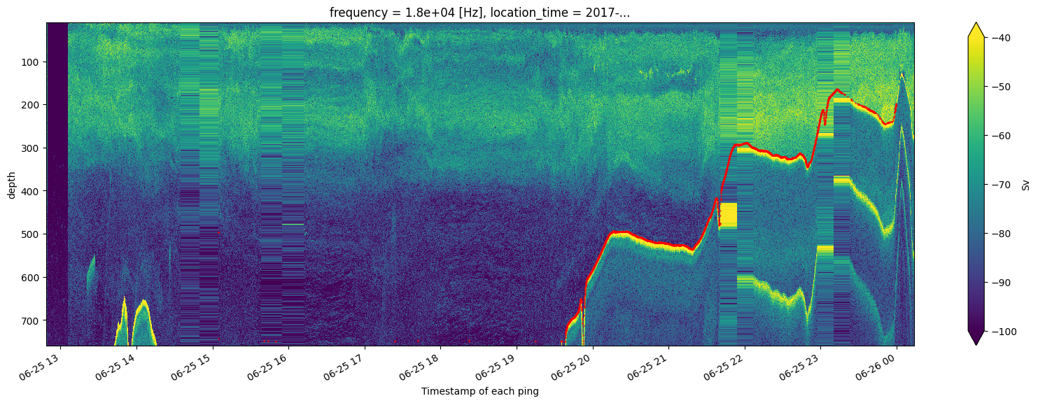
This notebook read bottom values from an Echoview .evl file and plots them superimposed on the corresponing sonar data.

# importing packages
import matplotlib.pyplot as plt
import os
import urllib.request
import dask

import echoregions as er

Bottom Data Reading

# path to evl files
TEST_DATA_PATH = 'https://raw.githubusercontent.com/OSOceanAcoustics/echoregions/main/echoregions/test_data'

# download an example file
urllib.request.urlretrieve("https://raw.githubusercontent.com/OSOceanAcoustics/echoregions/main/echoregions/test_data/x1.evr","x1.evr")

# read an example .evl file
line = er.read_evl('x1.evl')
line

<echoregions.formats.lines.Lines at 0x1ef21e55bd0>

Line as a DataFrame

line is a specialized object but it has a data attribute which is a simple dataframe.

# store the object's data in a dataframe
line_df = line.data

line_df

	file_name	file_type	evl_file_format_version	echoview_version	time	depth	status
0	x1	EVBD	3	12.0.341.42620	2017-06-25 15:04:28.137000	496.834625	1
1	x1	EVBD	3	12.0.341.42620	2017-06-25 15:04:28.137000	496.834625	3
2	x1	EVBD	3	12.0.341.42620	2017-06-25 15:04:35.895000	496.838999	3
3	x1	EVBD	3	12.0.341.42620	2017-06-25 15:04:35.896000	743.307494	3
4	x1	EVBD	3	12.0.341.42620	2017-06-25 15:40:43.910500	748.760741	3
...	...	...	...	...	...	...	...
7100	x1	EVBD	3	12.0.341.42620	2017-06-26 02:19:56.994000	84.898303	3
7101	x1	EVBD	3	12.0.341.42620	2017-06-26 02:19:59.818000	84.860518	3
7102	x1	EVBD	3	12.0.341.42620	2017-06-26 02:20:02.699000	85.528454	3
7103	x1	EVBD	3	12.0.341.42620	2017-06-26 02:20:05.572000	85.472250	3
7104	x1	EVBD	3	12.0.341.42620	2017-06-26 02:20:08.443000	85.260804	0

7105 rows × 7 columns

# status 3 are good points
line_df = line_df[line_df['status']=='3']

# extract only the ping_time and depth columns
bottom = line_df[['time','depth']]
bottom

	time	depth
1	2017-06-25 15:04:28.137000	496.834625
2	2017-06-25 15:04:35.895000	496.838999
3	2017-06-25 15:04:35.896000	743.307494
4	2017-06-25 15:40:43.910500	748.760741
5	2017-06-25 15:40:43.911500	748.110964
...	...	...
7099	2017-06-26 02:19:54.169000	85.091041
7100	2017-06-26 02:19:56.994000	84.898303
7101	2017-06-26 02:19:59.818000	84.860518
7102	2017-06-26 02:20:02.699000	85.528454
7103	2017-06-26 02:20:05.572000	85.472250

5245 rows × 2 columns

plt.plot(bottom['time'], bottom['depth'],'r.')
plt.gca().invert_yaxis()

Sonar Data Reading

Here we will plot the backscatter for the set of files we have stored on Google Drive. We will just look at one frequency for simplicity.

# mounting the google drive (uncomment if you have permission to read directly from Google Drive)
# from google.colab import drive
# drive.mount('/content/drive/') 

# Paths for Google Drive read  (uncomment if you have permission to read directly from Google Drive)
# SONAR_PATH_Sv = '/content/drive/Shareddrives/uw-echospace/shared_data/SH1707/sample/Sv/'
# SONAR_PATH_raw = '/content/drive/Shareddrives/uw-echospace/shared_data/SH1707/sample/raw_converted'

# download a zipped sample folder from publicly available Google Drive
import gdown

url = 'https://drive.google.com/uc?id=1rPO8NaXS9cGtl0ex4KIc7HmT2PnXPg0S'
output = 'sample.zip'
gdown.download(url, output, quiet=False)

# Unzip into sample folder labeled "/sample"
import zipfile
with zipfile.ZipFile("sample.zip", 'r') as zip_ref:
    zip_ref.extractall()

# Paths for local read
SONAR_PATH_Sv = './sample/Sv/'
SONAR_PATH_raw = './sample/raw_converted/'

import xarray as xr

# reading the processed Sv data
ds_Sv = xr.open_mfdataset(os.path.join(SONAR_PATH_Sv, '*.nc'))

# reading the processed platform data
with dask.config.set(**{'array.slicing.split_large_chunks': True}):
    ds_plat = xr.open_mfdataset(os.path.join(SONAR_PATH_raw, '*.nc'), group='Platform')

# assuming water levels are same for different frequncies and location_time
depth = ds_plat.water_level.isel(location_time=0, frequency=0, ping_time=0)+ds_Sv.range.isel(frequency=0, ping_time=0)

# creating a new depth dimension
ds_Sv['depth'] = depth
ds_Sv = ds_Sv.swap_dims({'range_bin': 'depth'})

Plotting Sonar and Bottom

# plotting the sonar data and the bottom
plt.figure(figsize = (20, 6))
ds_Sv.Sv.isel(frequency=0).T.plot(yincrease=False, vmax=-40, vmin=-100)
plt.plot(bottom['time'], bottom['depth'],'ro',fillstyle='full', markersize=1)

[<matplotlib.lines.Line2D at 0x2a07bbf15a0>]

# plot filled bottom
plt.figure(figsize = (20, 6))
ds_Sv.Sv.isel(frequency=0).T.plot(yincrease=False, vmax=-40, vmin=-100)
plt.plot(bottom['time'], bottom['depth'],'ro',fillstyle='full', markersize=1)
plt.fill_between(bottom['time'], ds_Sv.Sv.depth.max(), bottom['depth'], interpolate = False)

<matplotlib.collections.PolyCollection at 0x2a0739a0eb0>

Note that this filling interpolates between the points which is not desirable when the bottom points are very sparse.

Plotting with line’s Built-in Plotting Method

The line object has a built-in plotting method which can shorten the above steps.

help(line.plot)

Help on method plot in module echoregions.formats.lines:

plot(fmt='', start_time=None, end_time=None, fill_between=False, max_depth=0, **kwargs) method of echoregions.formats.lines.Lines instance
    Plot the points in the EVL file.
    
    Parameters
    ----------
    fmt : str, optional
        A format string such as 'bo' for blue circles.
        See matplotlib documentation for more information.
    start_time : datetime64, default ``None``
        Lower time bound.
    end_time : datetime64, default ``None``
        Upper time bound.
    fill_between : bool, default True
        Use matplotlib `fill_between` to plot the line.
        The area between the EVL points and `max_depth` will be filled in.
    max_depth : float, default 0
        The `fill_between` function will color in the area betwen the points and
        this depth value given in meters.
    alpha : float, default 0.5
        Opacity of the plot
    kwargs : keyword arguments
        Additional arguments passed to matplotlib `plot` or `fill_between`.
        Useful arguments include `color`, `lw`, and `marker`.

from datetime import datetime

# making starting and ending times
start_time = datetime(2017, 6, 25)
end_time = datetime(2017, 6, 26)

plt.figure(figsize = (20, 6))
ds_Sv.Sv.isel(frequency=0).T.plot(yincrease=False, vmax=-40, vmin=-100)
line.plot(start_time=start_time, end_time=end_time, fill_between=False, linestyle='', marker='.', color='r', markersize=1)

c:\Users\cmtug\OneDrive\Documents\GitHub\echoregions\.venv\lib\site-packages\echoregions\plot\line_plot.py:29: UserWarning: linestyle is redundantly defined by the 'linestyle' keyword argument and the fmt string "" (-> linestyle='-'). The keyword argument will take precedence.
  plt.plot(df.time, df.depth, fmt, **kwargs)